The Roofline for LLMs: Why Decode Is Memory-Bound
"Decode is memory-bound" is the most repeated sentence in inference engineering, and it explains most of the series so far: why engines batch, why 4-bit weights make decoding faster, why speculative decoding works at all. This piece makes it concrete. With two numbers from a GPU's spec sheet and two from a model's config, you can say where any step sits, predict roughly how fast it will run, and see which optimization can help before you try it. Then we check the prediction against a real engine.
Two numbers per GPU
Every GPU has a peak compute rate, in floating-point operations per second (FLOPS), and a memory bandwidth, in bytes per second. A step of a model needs some number of operations and some number of bytes read from memory. Whichever of the two takes longer sets the time of the step:
time ≥ max( FLOPs / peak FLOPS , bytes / bandwidth )
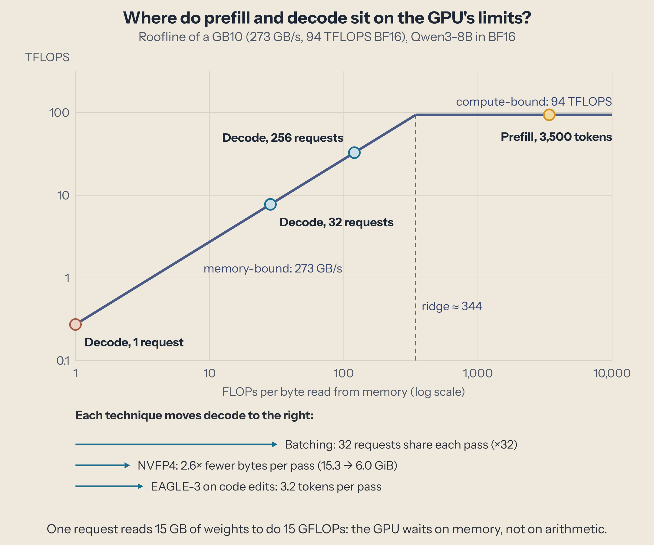
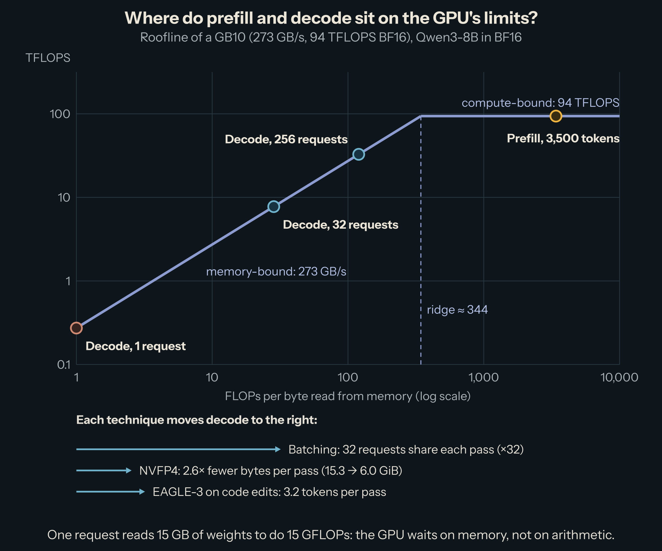
Divide the FLOPs by the bytes and you get the step's arithmetic intensity, in FLOPs per byte. Divide the GPU's peak by its bandwidth and you get its ridge: the intensity at which both limits take the same time. Below the ridge, the step waits on memory; above it, on arithmetic. Plotted on log axes, the best achievable rate is a slope that rises with intensity and then a flat roof: a roofline.
| GPU | Memory bandwidth | BF16, dense | Ridge (BF16) |
|---|---|---|---|
| RTX 5090 | 1.8 TB/s | 209.5 TFLOPS | 117 FLOPs/byte |
| H200 | 4.8 TB/s | 989 TFLOPS | 206 |
| B200 | 8 TB/s | 2,250 TFLOPS | 281 |
| MI355X | 8 TB/s | 2,517 TFLOPS | 315 |
| Rubin | 22 TB/s | 4,000 TFLOPS | 182 |
| GB10 (DGX Spark) | 273 GB/s | 94 TFLOPS (measured) | 344 |
Vendor specifications, dense (no sparsity), one GPU. NVIDIA does not publish a dense BF16 figure for the GB10, so that row uses the rate we measured (below).
Two things stand out. Every ridge is in the hundreds: a step must do hundreds of operations for each byte it reads to use the arithmetic fully. And no generation escapes it: Rubin nearly triples the B200's bandwidth, and its BF16 ridge is still 182. A step that does 1 FLOP per byte is memory-bound on every GPU in the table.
How many FLOPs per byte does a step do?
Take Qwen3-8B in BF16: 8.2 billion parameters, 2 bytes each, so 16.4 GB of weights. One table, the input embeddings (0.6 billion parameters), is only looked up, one row per token; everything else, 7.6 billion parameters or 15.1 GB, takes part in every token.
Decode, one request. Each new token passes through those weights once: a multiply and an add per parameter, 2 FLOPs, so 15.1 GFLOPs per token. And each of them must be read from memory once per step: 15.1 GB. That is 1 FLOP per byte, about 300 times below any ridge in the table. The arithmetic units are idle more than 99% of the time; the step's speed is the speed at which the weights stream from memory. On a GPU with 273 GB/s, that is 15.1 / 273 = 55 ms per token at best; on an H200, 3.2 ms.
Decode, a batch of requests. With 32 requests in the batch, each weight read from memory serves 32 tokens: 32 times the FLOPs for nearly the same bytes. Intensity rises to about 32. This is the whole reason continuous batching exists: batching is free throughput until the step reaches the ridge.
Prefill. Reading a 3,500-token prompt runs all 3,500 tokens through the weights in one pass: about 3,500 × 13.9 GFLOPs (the output layer runs only for the last token) for one read of the weights. Intensity is in the thousands, past every ridge: prompt reading is limited by arithmetic.
The part batching cannot share
Batching shares the weights, not the KV cache. Every request has its own cache, and every decode step reads all of it: for Qwen3-8B, 144 KiB per token of context (sized here). The attention that uses it does few operations per byte: for each cached token, 4 FLOPs per query head and dimension (a dot product for the score, a multiply-add for the weighted sum), over 4 bytes per KV head and dimension (a key and a value, 2 bytes each). With 32 query heads sharing 8 KV heads, attention runs at about 4 FLOPs per byte, whatever the batch size.
So decode intensity does not grow with the batch forever. With 256 requests of 384 tokens each, the caches add 14.5 GB to the 15.1 GB of weights, and intensity is about 130, not 256. With long contexts, the cache dominates, and decode is pinned close to the attention's 4 FLOPs per byte. This is why grouped-query attention, multi-head latent attention, and FP8 KV caches matter so much: they cut the bytes of the part batching cannot amortize.
Try it
Pick a GPU, a model, a weight format, and a phase; move the batch size and the context; the dot shows where one step lands, and the cards give the ideal time per step.
Three things to try:
- Decode on the H200 with 512 tokens of context, batch 1, then 64. The step time grows by about a third while tokens per second grow almost fifty-fold: the weights dominate what is read, so more requests are nearly free.
- Batch 256, context from 512 to 32,768. The dot slides back down the slope as the KV cache takes over: long contexts make batching pay less.
- Switch the weights from BF16 to FP4 on the B200. The roof rises fourfold and the bytes per weight shrink 3.6 times: decode with few requests runs about 3.5 times faster in this ideal model (2.7 times measured on Qwen3-8B, whose embeddings stay in BF16), and prefill climbs to a higher roof.
Measured: does a real engine follow the line?
A roofline is an upper bound. To see how close a real engine gets, we measured on an NVIDIA GB10 (DGX Spark), 2026-10-06, with vLLM 0.31.0 and PyTorch 2.13.
The two limits. First, the GPU's real peaks, with plain PyTorch:
a = torch.randn(n, n, device="cuda", dtype=torch.bfloat16); b = torch.randn(n, n, device="cuda", dtype=torch.bfloat16)
s = timeit(lambda: a @ b)
out[f"bf16_matmul_{n}_tflops"] = 2 * n**3 / s / 1e12
...
s = timeit(lambda: x.sum())
out["read_2gib_gbps"] = x.numel() * 2 / s / 1e9
{"device": "NVIDIA GB10", "torch": "2.13.0+cu132",
 "bf16_matmul_4096_tflops": 82.73, "bf16_matmul_8192_tflops": 93.78,
 "copy_2gib_gbps": 223.1, "read_2gib_gbps": 241.4}
A large BF16 matrix multiplication reaches 94 TFLOPS. Reading 2 GiB reaches 241 GB/s, 88% of the 273 GB/s specification, which is typical: the spec is the raw rate of the memory chips, and no kernel reads at exactly that rate.
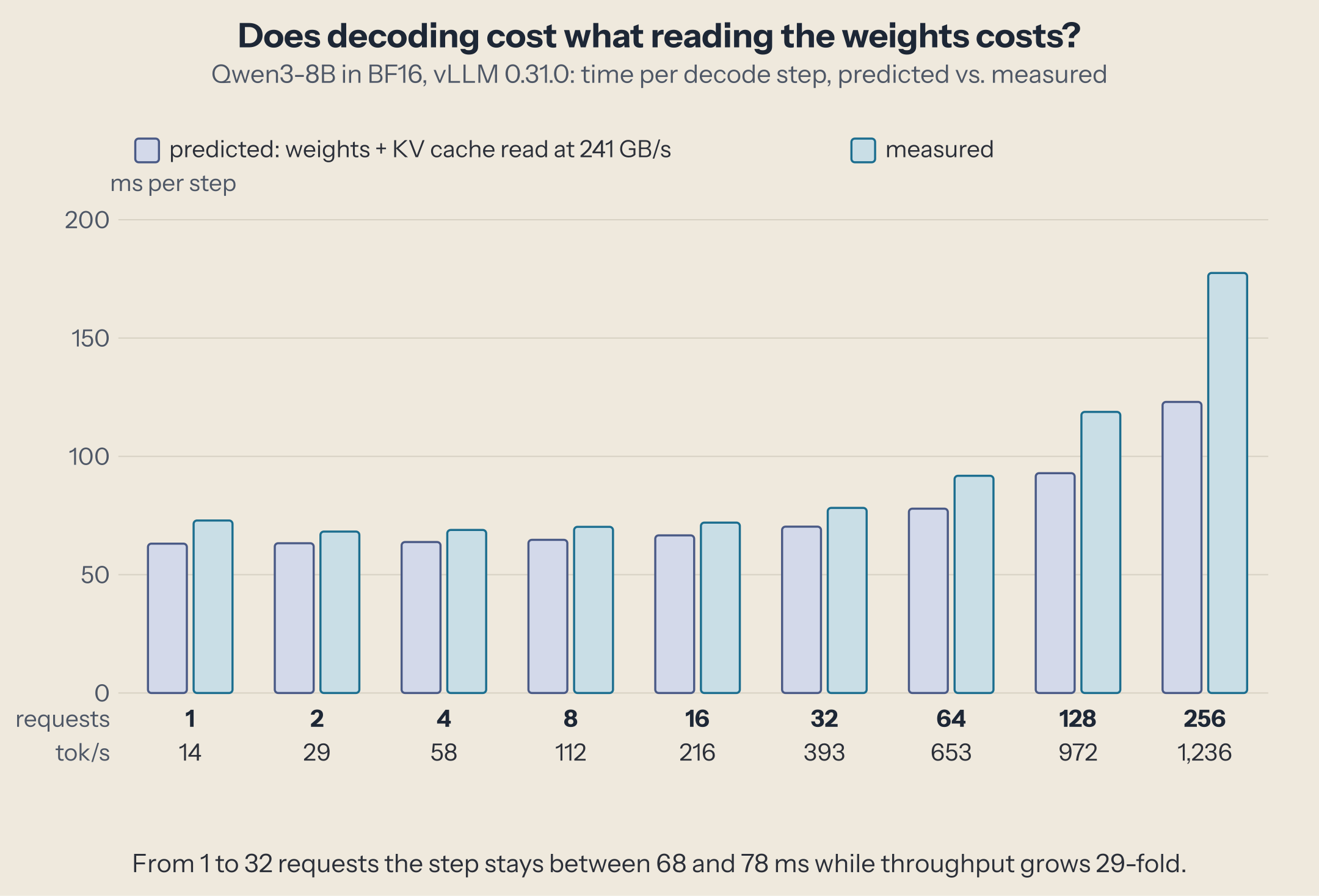
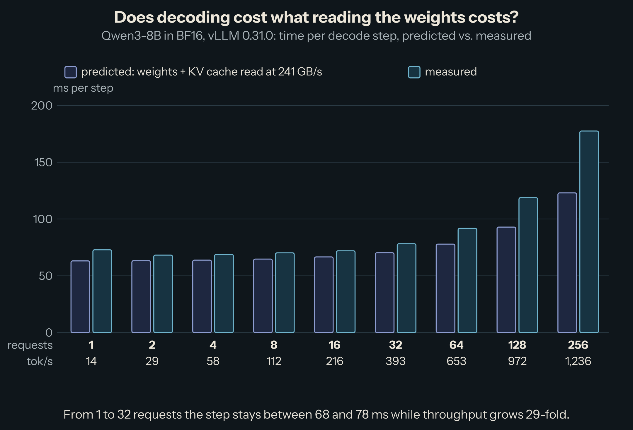
Decode, from 1 to 256 requests. Then Qwen3-8B in BF16, served with vLLM, at fixed concurrency from 1 to 256 (256-token prompts, 256-token answers, so about 384 tokens of context on average). The prediction uses the measured 241 GB/s: weights plus each request's KV cache, divided by bandwidth.
| Requests | Predicted step | Measured step (median) | Tokens/s, total |
|---|---|---|---|
| 1 | 63 ms | 73 ms | 13.7 |
| 2 | 63 ms | 68 ms | 29.1 |
| 4 | 64 ms | 69 ms | 57.7 |
| 8 | 65 ms | 70 ms | 112 |
| 16 | 67 ms | 72 ms | 216 |
| 32 | 70 ms | 78 ms | 393 |
| 64 | 78 ms | 92 ms | 653 |
| 128 | 93 ms | 119 ms | 972 |
| 256 | 123 ms | 178 ms | 1,236 |
All 2,064 requests completed, none failed.
What it shows:
- With few requests, the prediction holds, plus a constant. From 2 to 16 requests, every step costs the predicted read time plus about 5 ms: matrix-vector and attention kernels that read below the 241 GB/s of a plain read, plus sampling and the scheduler. Launching the step's kernels is a small part of it: vLLM replays most of them from CUDA graphs, under 1 µs each on this GPU, so its roughly 145 matrix kernels cost about 0.1 ms (a GPU in one picture). A lone request is the odd one out at 73 ms; the continuous batching piece measured the same 72 ms on an earlier vLLM release.
- Up to about 32 requests, tokens are almost free. The step stays between 68 and 78 ms while throughput grows 29-fold. This is the bottom of the slope: the same weight read now serves 32 tokens.
- Past 64 requests, the step costs more than its reads. 178 ms measured against 123 predicted at 256 requests. The arithmetic is no longer negligible: in this workload, every request that finishes is replaced by a new 256-token prompt, so each step also reads about one prompt token per answer token. At 256 requests, that is roughly 512 tokens through the weights per step, 7.7 TFLOPs, about 80 ms even at the full 94 TFLOPS. Reads and arithmetic do not overlap perfectly, and kernels run below their peak at these shapes: the measured time falls between the larger of the two (123 ms) and their sum (205 ms).
- Throughput still grows, but by less. Doubling from 128 to 256 requests gave 27% more tokens per second, against 49% from 64 to 128. Each answer's tokens arrive 2.4 times slower than with one request (178 against 73 ms). This is the trade-off that a serving configuration picks a point on.
- Decode alone never reaches the ridge. At 256 requests, decode's own intensity is about 130 FLOPs per byte, a third of the GB10's ridge: the KV cache keeps it down. What pushed the step toward the compute limit was the prompts mixed into it.
Prefill. A lone 3,500-token prompt took 685 ms to its first token (median of 8, within 4 ms of each other): 5,100 prompt tokens per second. Counting only what the prompt really computes (the output layer runs for the last token only), that is about 52 TFLOPs in 685 ms, 76 TFLOPS, 81% of the matrix-multiplication peak. Prompt reading sits on the flat part of the roof, as predicted, and it runs close to it.
The series, on one chart
Every technique in this series either moves a step to the right (more FLOPs per byte), lowers the bytes or FLOPs a step needs, or keeps the two kinds of steps from getting in each other's way.
- Continuous batching moves decode to the right: one weight read serves every request in the batch. The cheapest gain there is, until the KV cache takes over.
- Quantized weights cut the bytes. For decode, fewer bytes means proportionally faster steps: Qwen3-8B went from 15.3 to 6.0 GiB in NVFP4 and decoded 2.7 times faster with one request. With 4-bit tensor cores (W4A4), the roof rises too, so prefill also speeds up.
- FP8 KV caches and grouped-query attention cut the bytes batching cannot share.
- Speculative decoding spends the idle arithmetic: the big model verifies several drafted tokens per weight read, up to 3.2 tokens per pass in our runs. It helps most where decode sits lowest on the slope, which is why its speed-up falls as the batch grows.
- Chunked prefill mixes a compute-bound prompt chunk with memory-bound decode tokens in one step: the step uses both limits instead of one.
- Prefix caching removes prefill FLOPs altogether for tokens already seen.
- Disaggregated serving puts the two regimes on separate GPUs, so each can be sized and tuned for its own limit.
Where the roofline stops being enough
The roofline gives an upper bound and a direction. It does not predict everything:
- Overheads. The scheduler, sampling, and kernel launches cost time per step no matter the bytes: without CUDA graphs, about 3 µs per launch and hundreds of launches per step. For small models on fast GPUs, where the ideal step is 1 or 2 ms, they can dominate.
- Kernel efficiency. The line assumes every kernel runs at the peak. Attention kernels, small matrix shapes, and odd formats often do not.
- Mixture of experts. Only the active experts are read per token, but with a batch, different tokens pick different experts: the bytes per step grow with the batch until all experts are read.
- Capacity. The roofline says nothing about whether the weights and the KV cache fit. A batch of 256 is only possible if memory holds 256 caches.
- Several GPUs. With tensor parallelism, communication between GPUs adds a third limit, the interconnect, with its own ridge.
Next
The roofline explains what a GPU is waiting on; the next step is to see what happens inside the kernels that do the waiting. That is where the CUDA course starts.
This post is part of the The GPU for Inference Engineers collection (2 of 3)

Inference engineering and AI in production — depth-first, no hype.
Inference Notes
Once a week: what changed in serving AI models, and what it means if you build, run or pay for them, in about five minutes.
Related Articles
DeepGEMM: The Matrix Multiplications Behind DeepSeek's Models
What DeepGEMM computes for DeepSeek's models: block-scaled FP8 and FP4 matrix multiplications, grouped GEMMs for MoE experts, and the fused Mega MoE kernel.
Your First CUDA Kernel, Compiled and Profiled
Write SAXPY in CUDA, compile it for a Blackwell GPU, check it, time it, and read what Nsight Systems and Nsight Compute say about it.
A GPU in One Picture: SMs, Warps, and Memory
The parts of a GPU that decide inference speed, from streaming multiprocessors to DRAM, with one real GPU's numbers and three measurements.